Interpolating covariances with their geometric mean

What’s the best way to quantify and visualize distance between two positive definite matrices? Julia code included.

How should we incrementally transform (interpolate) between two Gaussian distributions with covariance matrices \(C_1\) and \(C_2\)? This question is deeply related to optimal transport, and Wasserstein distance, topics that have become popular in ML in recent years.

One possibility is to take a weighted arithmetic mean between the two covariances, \(C_{\text{interp}}(t) = (1-t)C_1 + tC_2\), where \(t\) is between zero and one. This is what’s shown on the left below (red \(\rightarrow\) yellow), but it turns out that this is suboptimal.

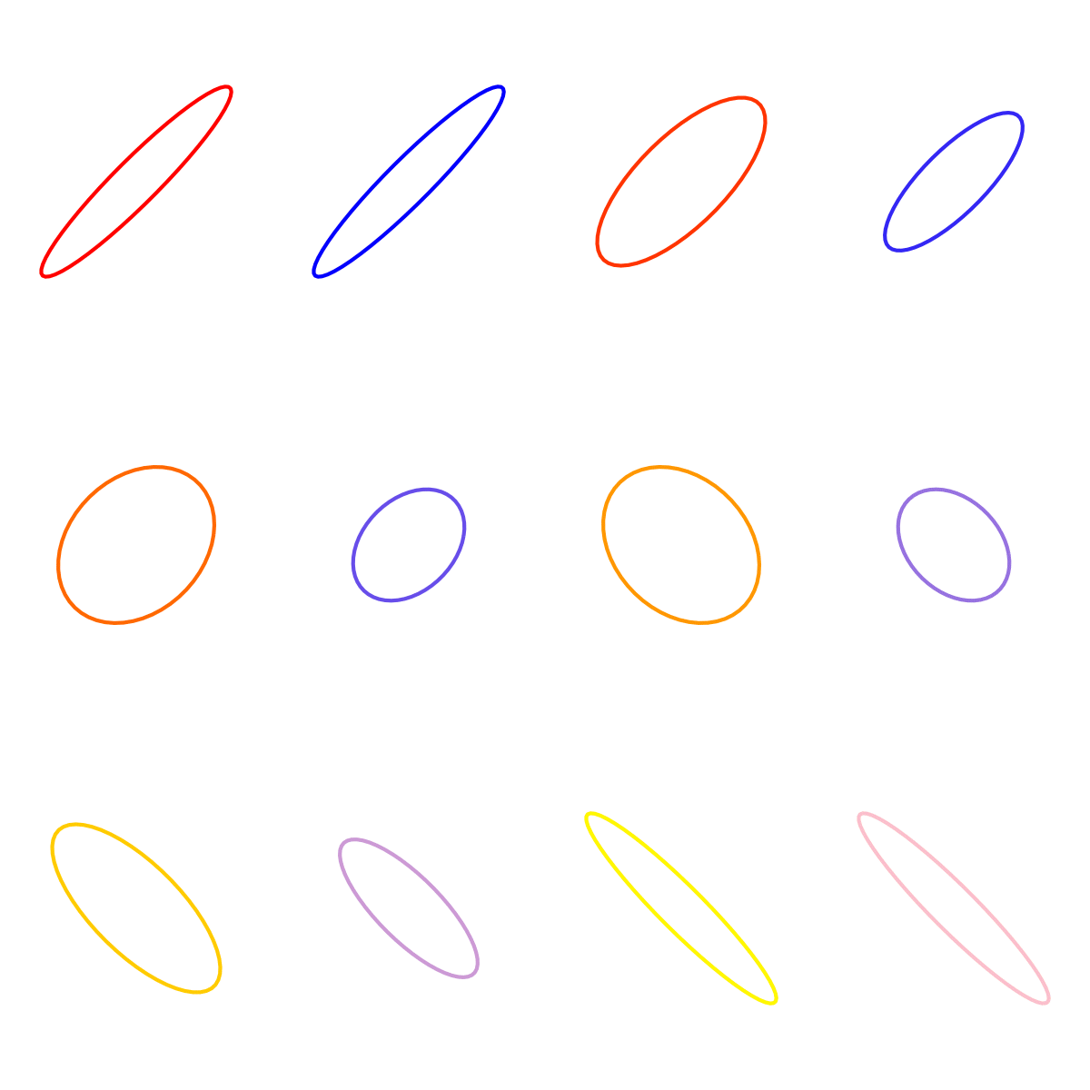
The left ellipse inflates like a balloon in transforming from \(C_1\) to \(C_2\). Alternatively, the geometric mean is a more natural distance to travel, \(C_{\text{interp}}(t)=C_1^{1/2} \left(C_1^{-1/2} C_2 C_1^{-1/2}\right)^t C_1^{1/2}\). The right panel above shows the interpolation between the same two covariances as before, but this time using the weighted geometric mean.

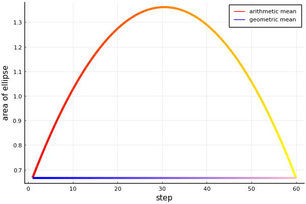
Using the geometric mean, the ellipse no longer swells up during the transformation. In fact, the area doesn’t change at all, as you can see in the fig below. The colours of the lines correspond to the colours of the ellipses in the first fig.

Any symmetric matrix \(\begin{bmatrix} \sigma_x^2 & \sigma_{xy} \\ \sigma_{xy} & \sigma_y^2 \end{bmatrix}\) is only a covariance matrix if it is positive definite, which in the 2x2 case means \(\sigma_{xy}^2 < \sigma_x^2\sigma_y^2\). Geometrically, this inequality traces out a cone (x axis is \(\sigma_x\), y axis is \(\sigma_y\), and z axis is \(\sigma_{xy}\)). Below, you can see the trajectories from the arithmetic and geometric covariance interpolations in this positive definite cone.

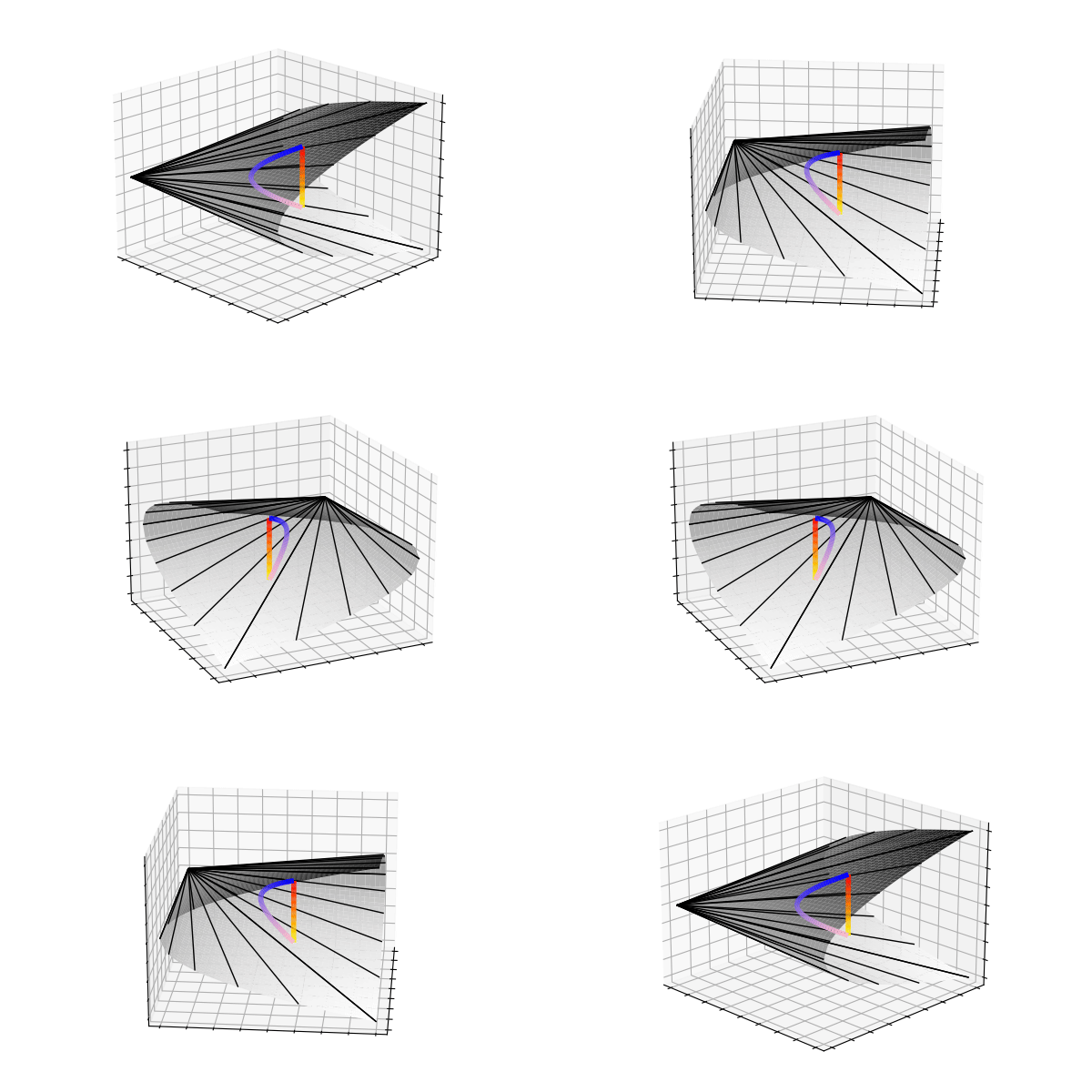
So, despite the arithmetic-mean trajectory (red\(\rightarrow\)yellow) tracing out a straight-line, the highly curved geometric-mean trajectory (blue\(\rightarrow\)pink) unintuitively leads to the nicer interpolation we saw at the beginning. It turns out that, moving along the weighted geometric mean is the equivalent to traversing the unique geodesic between the two points on the manifold of covariance matrices.